- File Setup for Selective U Application
Important: When applying Hubbard U corrections to only some atoms of the same element type (e.g., applying +U to only some U atoms in URhGe), you must modify both POSCAR and POTCAR files to distinguish between atoms that receive the correction and those that don't.
Example for URhGe system:
If your original POSCAR has:
URhGe
4.0
...
U  Rh  Ge
4  4   4
And you want to apply +U to only the first U atom, modify it to:
URhGe
4.0
...
U  U   Rh  Ge
1  3   4   4
This creates two distinct "U" species: the first one (1 atom) will receive the +U correction, and the second one (3 atoms) will be treated as regular U atoms.
Correspondingly, your POTCAR file must be created with:
potcreate U U Rh Ge
This ensures that VASP recognizes four distinct atomic species, allowing you to apply different parameters to each.
With this setup, your LDA+U parameters would be:
LDAU         = .TRUE.
LDAUTYPE     = 3
LDAUL        = 3  -1  -1  -1     # Apply to f-orbitals of 1st U only
LDAUU        = 3.42 0.00 0.00 0.00  # U parameter only for 1st U species
LDAUJ        = 0.51 0.00 0.00 0.00  # J parameter only for 1st U species
The first set of parameters applies to the first U species (receiving +U), while the remaining parameters apply to the second U species, Rh, and Ge respectively (all set to not receive corrections).
- Ground State Calculation
Prepare the required input files for your system. The example below shows NiO with antiferromagnetic ordering, but the approach applies similarly to other systems like UGe₂.
POSCAR setup (following the file setup from step 1):
For NiO where you want to apply +U to all Ni atoms but distinguish different magnetic sites:
NiO AFM
4.03500000
2.0000000000   1.0000000000   1.0000000000
1.0000000000   2.0000000000   1.0000000000
1.0000000000   1.0000000000   2.0000000000
Ni  Ni  O
1   15   16 (adding one more Ni species to distinguish sites, so total 2 Ni species)
Direct
...atomic positions...
POTCAR setup:
Create the POTCAR file with distinct entries for each species defined in POSCAR:
potcreate Ni Ni O
INCAR file for ground state calculation:
    SYSTEM       = NiO AFM
    PREC         = A
    EDIFF        = 1E-6
    ISMEAR       = 0
    SIGMA        = 0.2
    ISPIN        = 2
    MAGMOM       = 1.0 -1.0  1.0 -1.0  \
                1.0 -1.0  1.0 -1.0  \
                1.0 -1.0  1.0 -1.0  \
                1.0 -1.0  1.0 -1.0  \
                16*0.0
    LORBIT       = 11
    LMAXMIX      = 4
This run provides the reference ground state charge density and wavefunction (CHGCAR, WAVECAR).
- NSCF Step
Copy the following from the ground state directory:
POSCARPOTCARINCARKPOINTSWAVECAR and CHGCAR
Then add the following line to INCAR for the NSCF step:
ICHARG = 11
Also append these LDA+U parameters (example for Ni with U and J = 0.10 eV, where only the first Ni species receives the correction):
    LDAU         = .TRUE.
    LDAUTYPE     = 3
    LDAUL        = 2 -1 -1           # Apply to d-orbitals of Ni 1
    LDAUU        = 0.10 0.00 0.00   # U parameter for Ni 1
    LDAUJ        = 0.10 0.00 0.00   # J parameter for Ni 1
In this example, the correction is applied to the first atom (Ni, 3d orbital). Adjust accordingly for your system.
- SCF Step
From the NSCF run, copy:
POSCARPOTCARINCARKPOINTSWAVECAR
Remove ICHARG = 11 from INCAR for the SCF run.
- File Setup Note
The file setup described above is crucial for proper Hubbard U calculations. The POSCAR and POTCAR files must reflect the distinction between atomic species that receive different treatments, even if they are chemically identical atoms.
    TITEL  = PAW Ni 02Aug2007
    TITEL  = PAW Ni 02Aug2007
    TITEL  = PAW O  22Mar2012
    AFM  NiO
    4.03500000
    2.0000000000   1.0000000000   1.0000000000
    1.0000000000   2.0000000000   1.0000000000
    1.0000000000   1.0000000000   2.0000000000
    1 15   16
- Parameter Sweep
Repeat NSCF and SCF runs for the following U = J values:
0.15, 0.20, 0.05, 0.00, -0.05, -0.10, -0.15, -0.20 eV
- Analysis
After obtaining the number of localized electrons (e.g., f or d orbital) for each run, perform linear response fitting using Python:
    import numpy as np
    import matplotlib.pyplot as plt

    # Applied potential (eV)
    J = np.array([-0.1, -0.05, 0, 0.05, 0.1, 0.15, 0.2])

    # Number of f-electrons (example data)
    NSCF = np.array([2.182, 2.345, 2.517, 2.697, 2.885, 3.08, 3.282])
    SCF  = np.array([2.448, 2.461, 2.520, 2.533, 2.548, 2.563, 2.575])

    # Fit linear response (n vs J)
    s_n, intercept_n = np.polyfit(J, NSCF, 1)
    s_s, intercept_s = np.polyfit(J, SCF, 1)

    U = 1.0/s_s - 1.0/s_n

    # Generate fits
    J_fit = np.linspace(J.min(), J.max(), 200)
    fit_NSCF = s_n * J_fit + intercept_n
    fit_SCF  = s_s * J_fit + intercept_s

    # Print results
    print(f"chi0 (NSCF slope) = {s_n:.4f}")
    print(f"chi  (SCF slope)  = {s_s:.4f}")
    print(f"U (eV)            = {U:.4f}")

    # Plot (like VASP wiki)
    plt.figure(figsize=(7,5))
    plt.scatter(J, NSCF, color='black', label='NSCF', marker='o', facecolors='none', s=70)
    plt.scatter(J, SCF,  color='red', label='SCF',  marker='s', s=60)
    plt.plot(J_fit, fit_NSCF, color='black', linestyle='-', label=f'NSCF fit (χ₀={s_n:.3f})')
    plt.plot(J_fit, fit_SCF,  color='red', linestyle='-', label=f'SCF fit (χ={s_s:.3f})')
    plt.xlabel("Applied potential J (eV)")
    plt.ylabel("Number of f-electrons")
    plt.title("Linear Response for Hubbard U Determination of UGe₂")
    plt.grid(True, linestyle=':')
    plt.legend()
    plt.tight_layout()
    plt.show()
Example output:
    chi0 (NSCF slope) = 3.6700
    chi  (SCF slope)  = 0.4379
    U (eV)            = 2.0114
This method extracts the on-site Coulomb interaction U via linear response by comparing self-consistent and non-self-consistent changes in orbital occupations with applied potential perturbations.